Contents

How to filter data in pivot tables

You can use various types of filtering to display only required data in a pivot table.

The guide describes the following topics:

• Filtering data
• Filtering values in the field
• Create a filtering condition in the Prefilter dialog
• Editing and removing filters

Filtering data

You can filter all data in the pivot table by a specific field or by values.

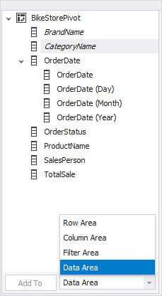
To filter data by a specific field, drag the field from the Data Source pane to Drop Filter Fields Here in the Pivot Table view.

Alternatively, in the Data Source pane, select the field by which you want to filter data. At the bottom of the pane, select Filter Area from the dropdown list and click Add to. However, this can be done only after you have already added data, rows, and columns to the pivot table.

To filter data by values:

1. Click Filter on the data header control

2. In the dialog that opens, enter the values in the Show values from/to input fields or move the filter bar to the left or right.

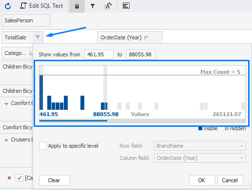
3. If you want to filter values at a specific level, select the Apply to specific level checkbox and do the following:

• Enter the values you want to display in the input fields.
• Select the row and column fields from the dropdown lists.

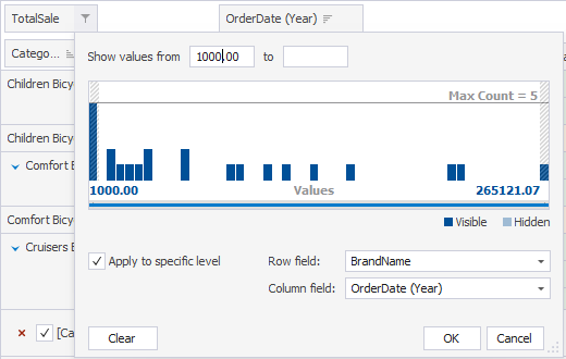
4. Click OK to apply the filter.

Filtering values in the field

You can filter text and numeric values in the row and column fields.

To filter text values:

1. Click Filter on the header control.

2. In the Values dialog that opens, select the values that you want to display.

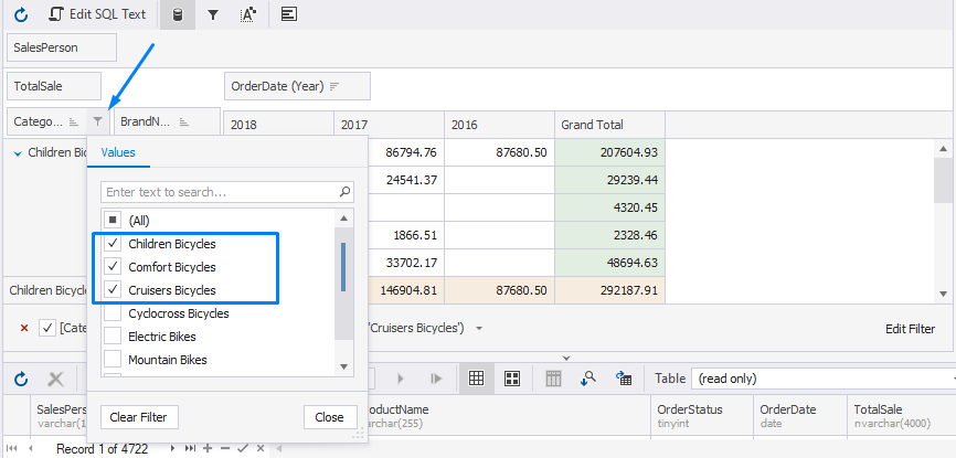
3. In the Values dialog, you can also search for the required value. For this, start typing the value. All the matching values will be highlighted and displayed under the search field.

To filter numeric values:

1. Click Filter on the header control with numeric values.

2. In the dialog that opens, switch to the Numeric Filters tab and do the following:

• From the first dropdown list, select the operator.

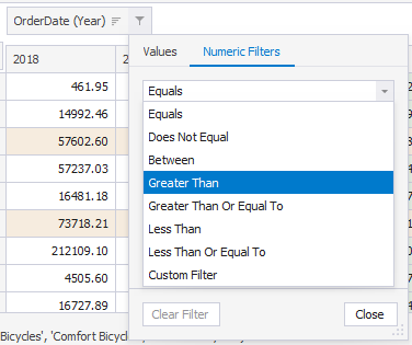
• From the second dropdown list, select the value. For example, bicycles that were ordered after 2017.

3. Click Close to close the dialog.

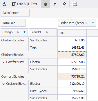
As a result, the pivot table now displays bicycles ordered for 2018.

Create a filtering condition in the Prefilter dialog

Also, you can use the PivotGrid Prefilter dialog to apply advanced filtering conditions to filter data.

1. To open the dialog, click Prefilter on the toolbar or right-click the pivot table header and select Prefilter.

2. In the PivotGrid Prefilter dialog that opens, click Add to add a new condition and do the following:

• Select the field name from the dropdown list.
• Click the condition criteria operator to select a required one from the drop-down list.
• Enter the value.

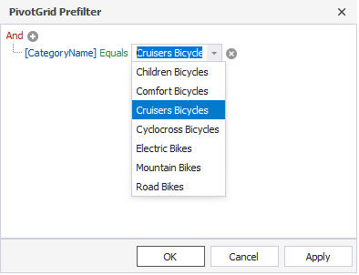
3. Click Apply and then OK to apply the filter.

4. To add more conditions to this group, click Add and specify the condition properties.

To remove a condition, click the condition icon or navigate to the condition and press DELETE.

5. To add a new group of conditions, click the upper-level group operator and select Add Group from the menu. Then, specify the condition properties. To remove a group, click its logical operator and select Remove Group from the menu.

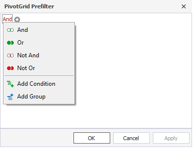
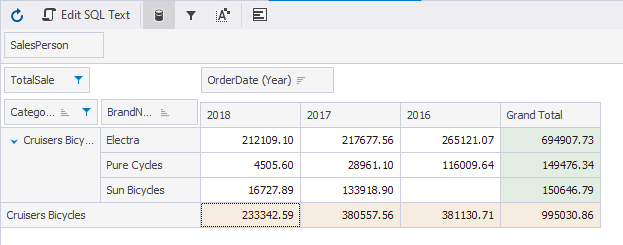
6. The pivot table will display data matching the created filtering conditions.

Editing and removing filters

To see the data unfiltered, clear the checkbox next to the filtering condition at the bottom of the Pivot Table view.

To edit filters, at the bottom of the Pivot Table view, click Edit Filter. This will open the Filter Editor dialog where you can edit filters.

To remove filters, at the bottom of the Pivot Table view, click Remove.

Want to Find out More?

• Previous
• Next