Applying Conditional Styles
Conditional styles give you freedom to change a pivot table appearance to make the data more readable. For example, you can highlight values of some field that are greater than 100 with the red color, and values of another field that meet some other condition with the blue color, the difference between data in a pivot table will be clear at a glance.
Besides setting a background color for some cells, you can select an image as a background, change a font and its color, specify a condition to apply only for some values in a required field, etc.
Let’s examine conditional styles benefits by the following example:
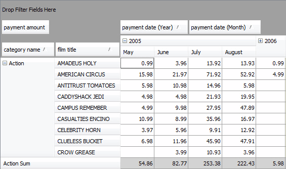
There is the list of films and their rental payments grouped by month and year. It is required to quickly identify which films bring the expected revenue, i.e., the sum of their rental payments meet the planned monthly range of $20-40 and which films are in less demand, i.e., the sum of their rental payments are less than $10.
Conditional styles in use:
- Open the Conditional Styles dialog box by either of these ways:
- Click the
 Conditional Styles icon on the toolbar
 - Right-click the pivot table header and select Conditional Styles on the menu
- Click the
- Click the
 Add Condition icon to create a new condition.
 - Select the payment amount field from the Field drop-down list and go to the Condition field to select the Between value.
- Enter 20 and 40 values into Value1 and Value2 fields to specify the required range of values.
- Clear all the check boxes except the Cell one in the Apply To section, as there is no need to apply this condition for all the cell types in the pivot table.
-
In the Appearance section, click the BackColor field and select LightBlue. Now, the first condition is ready. Click the
Add Condition icon to create another condition for the films which have the sum of payment amounts less than $10.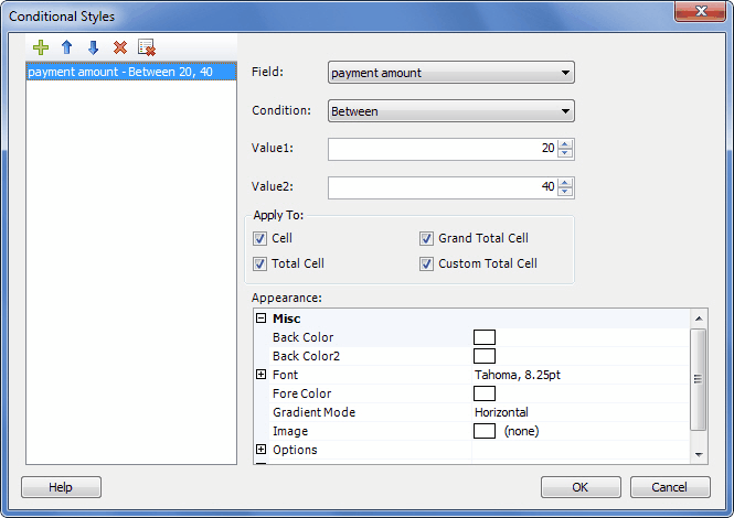
- Select the payment amount field from the Field drop-down list and go to the Condition field to select the Less value.
- Enter 10 into the Value1 field and leave only the Cell check box selected in the Apply To section.
- In the Appearance section, select the red color from the ForeColor field to change the font color of the payment amount values into red.
- Click OK to apply the conditional styles to the pivot table. The data will look like the following: